| Demand®
Order |
|
|
|
| Small |
|
|
|
| Medium |
|
|
|
| Large |
|
|
|
2.1 Introduction and Basic Terms
Decision theory represents a generalized approach to decision making. It enables the decision maker
Some examples of alternatives and possible
events for these alternatives are shown in Table 2.1.
|
|
|
| To order 10, 11, … units of a product | Demand for the product may be 0, 1, … units |
| To make or to buy a product | The cost of making may be 20, 22, …$thousands |
| To buy or not to buy accident insurance | An accident may occur, or may not occur |
Table 2.1 “Examples of Alternatives and Events”
Various properties of decision problems enable a classification of decision problems.
Solution to any decision problem consists of these steps:
Rows of a payoff table (called also decision matrix) relate to the alternatives, columns relate to the states of nature. Elements of a decision matrix represent the payoffs for each alternative under each possible event.
We will construct a payoff table for the following simple example.
A grocer solves a problem of how much pastry
to order every day. His profit depends on a demand that can be low, moderate,
or high. Values of the profit per day (in $) for these situations and for
small, medium or large order are shown in Table 2.2. The body of this table
represents a decision matrix.
| Demand®
Order |
|
|
|
| Small |
|
|
|
| Medium |
|
|
|
| Large |
|
|
|
Table 2.2 “Payoff Table for Order Planning”
The environments in which decisions are made can be classified according to the degree of certainty. There are three basic categories: certainty, risk, and uncertainty. The importance of these three decision environments is that they require different techniques of analysis.
2.2 Decision Making under Certainty
When the decision maker knows for certain which state of nature will occur, he will choose the alternative that has the highest payoff (or the smallest loss) under that state of nature.
In the above grocer´s decision problem, suppose that it is known with certainty that demand will be low. The highest profit for low demand is $50 (see Table 2.2) and therefore the small order should be elected.
2.3 Decision Making under Uncertainty
Under complete uncertainty, either no estimates of the probabilities for the occurrence of the different states of nature are available, or the decision maker lacks confidence in them. For that reason, probabilities are not used at the choice of the best alternative.
Most of the rules for decision making under uncertainty express a different degree of decision maker´s optimism.
We will describe the most used rules for the choice of the best alternative supposing that the decision criterion expresses the requirement of maximization (the modification of these rules for minimization criteria is not difficult). We will use all the described rules to solution of the order planning problem given in Table 2.2.
The maximax rule is appropriate
for extreme optimists that expect the most favourable situation (they choose
the alternative that could result in the maximum payoff). Under this rule,
the decision maker will find the largest payoff in the decision matrix
and select the alternative associated with it (the largest payoff is determined
for each alternative and then the largest payoff from these values is selected;
therefore “maximax”). This procedure for the order planning problem is
shown in Table 2.3.
| Demand®
Order |
|
|
|
|
|
| Small |
|
|
|
|
|
| Medium |
|
|
|
|
|
| Large |
|
|
|
|
|
Table 2.3 “Maximax Solution for Order Planning Problem”
The best overall profit is $54 in the third row. Hence, the maximax rule leads to the large order (the grocer hopes that the demand will be high).
The maximin rule (Wald criterion) represents a pessimistic approach when the worst decision results are expected. The decision maker determines the smallest payoff for each alternative and then chooses the alternative that has the best (maximum) of the worst (minimum) payoffs (therefore “maximin”).
In Table 2.2, the smallest numbers in the rows are 50, 42, 34. Since 50 is the largest, the low order should be chosen (if order is low, the $50 grocer‘s profit is guaranteed).
The Hurwicz![]() -criterion
represents a compromise between the optimistic and the pessimistic approach
to decision making under uncertainty. The measure of optimism and pessimism
is expressed by an optimism - pessimism index
-criterion
represents a compromise between the optimistic and the pessimistic approach
to decision making under uncertainty. The measure of optimism and pessimism
is expressed by an optimism - pessimism index![]() ,
, ![]()
![]() <0,1> . The more this index is near to 1, the more the decision maker
is optimist. By means of the index
<0,1> . The more this index is near to 1, the more the decision maker
is optimist. By means of the index ![]() ,
a weighted average of the best payoff (its weight =
,
a weighted average of the best payoff (its weight = ![]() )
and
the worst payoff (its weight = 1-
)
and
the worst payoff (its weight = 1-![]() )
is computed for each alternative and the alternative with the largest weighted
average should be chosen (see formula for Hurwicz
criterion).
)
is computed for each alternative and the alternative with the largest weighted
average should be chosen (see formula for Hurwicz
criterion).
If ![]() =1,
the above rule is the maximax criterion, whereas if
=1,
the above rule is the maximax criterion, whereas if ![]() =0,
it is the maximin rule.
=0,
it is the maximin rule.
If we choose ![]() =
0.7 at determining the best size of the order in Table 2.2, the weighted
average (WA) of the largest and the smallest profit for each size of the
order has the following values:
=
0.7 at determining the best size of the order in Table 2.2, the weighted
average (WA) of the largest and the smallest profit for each size of the
order has the following values:
WA (medium) = 0.7* 52 + 0.3 * 42 = 49
WA (large) = 0.7* 54 + 0.3 *34 = 48
The maximax and maximin rules and the Hurwicz criterion can be criticized because they focus only on extreme payoffs and exclude the other payoffs. An approach that does take all payoffs into account is the minimax regret rule (Savage criterion). This rule represents a pessimistic approach used for an opportunity loss table. The opportunity loss reflects the difference between each payoff and the best possible payoff in a column (it can be defined as the amount of profit foregone by not choosing the best alternative for each state of nature). Hence, opportunity loss amounts are found by identifying the greatest payoff in a column and, then, subtracting each of the other values in the column from that payoff. The values in an opportunity loss table can be viewed as potential ”regrets” that might be suffered as the result of choosing various alternatives. Minimizing the maximum possible regret requires identifying the maximum opportunity loss in each row and, then, choosing the alternative that would yield the minimum of those regrets (this alternative has the “best worst”).
To illustrate the described procedure, we will recall the decision problem given in Table 2.2 and first construct the corresponding regret table.
Payoff table:
| Demand®
Order |
|
|
|
| Small |
|
|
|
| Medium |
|
|
|
| Large |
|
|
|
In the first column of the payoff matrix,
the largest number is 50, so each of the three numbers in that column must
be subtracted from 50. In the second column, we must subtract each payoff
from 52 and in the third column from 54. The results of these calculations
are summarized in Table 2.4. A column with the maximum loss in each row
is added to this table.
| Demand®
Order |
|
|
|
|
|
| Small |
|
|
|
|
|
| Medium |
|
|
|
|
|
| Large |
|
|
|
|
Table 2.4 “Regret Table for Order Planning”
Minimizing the maximum loss, the small order should be chosen.
The minimax regret criterion disadvantage is the inability to factor row differences. It is removed in the further rule that incorporates more of information for the choice of the best alternative.
The principle of insufficient reason (Laplace criterion) assumes that all states of nature are equally likely. Under this assumption, the decision maker can compute the average payoff for each row (the sum of the possible consequences of each alternative is divided by the number of states of nature) and, then, select the alternative that has the highest row average. This procedure is illustrated by the following calculations with the data in Table 2.2.
EMV (small) = (50 + 50 + 50)/3 = 50
EMV (medium) = (42 + 52 + 52)/3 = 48 2/3
EMV (large) = (34 + 44 + 54)/3 = 44
Since the profits at the small order have the highest average, that order should be realized.
2.4 Decision Making under Risk
In this case, the decision maker doesn´t know which state of nature will occur but can estimate the probability of occurrence for each state. These probabilities may be subjective (they usually represent estimates from experts in a particular field), or they may reflect historical frequencies.
A widely used approach to decision making under risk is expected monetary value criterion.
The expected monetary value (EMV) of an alternative is calculated by multiplying each payoff that the alternative can yield by the probability for the relevant state of nature and summing the products. This value is computed for each alternative, and the one with the highest EMV is selected.
In the discussed grocer´s decision problem, suppose that the grocer can assign probabilities of low, moderate and high demand on the basis of his experience with sale of pastry. The estimates of these probabilities are 0.3, 0.5, 0.2, respectively. We will recall the payoff table for the considered problem.
Payoff table:
| Demand®
Order |
|
|
|
| Small |
|
|
|
| Medium |
|
|
|
| Large |
|
|
|
The EMV for various sizes of the order are as follows.
EMV (small) = 0.3*50 + 0.5*50 + 0.2*50 = 50
EMV (medium) = 0.3*42 + 0.5*52 + 0.2*52 = 49
EMV (large) = 0.3*34 + 0.5*44 + 0.2*54 = 43
Therefore, in accordance with the EMV criterion, the small order should be chosen.
Note that the EMV of $50 will not be the profit on any one day. It represents an expected or average profit. If the decision were repeated for many days (with the same probabilities), the grocer would make an average of $50 per day by ordering the small amount of pastry. Even if the decision were not repeated, the action with the highest EMV is the best alternative that the decision maker has available.
The EMV criterion remains as the most useful of all the decision criteria for decision making under risk. For risky decisions, a sensible approach is first to calculate the EMV, and then to make a subjective adjustment for the risk in making the choice.
Another method for incorporating probabilities into the decision making process is to use expected opportunity loss (EOL). The approach is nearly identical to the EMV approach, except that a table (or matrix) of opportunity losses (or regrets) is used. The opportunity losses for each alternative are weighted by the probabilities of their respective states of nature and these products are summed. The alternative with the smallest expected loss is selected as the best choice.
We will use this procedure in the regret matrix shown in Table 2.4. We will recall this table.
Regret table:
| Demand®
Order |
|
|
|
| Small |
|
|
|
| Medium |
|
|
|
| Large |
|
|
|
Supposing that the probabilities of various sizes of the demand are 0.3, 0.5, 0.2, we can determine the EOL for each size of the order.
EOL (small) = 0.3*0 + 0.5*2 + 0.2*4 = 1.8
EOL (medium) = 0.3*8 + 0.5*0 + 0.2*2 = 2.8
EOL (large) = 0.3*16 + 0.5*8 + 0.2*0 = 8.8
Since the small order is connected with the smallest EOL, it is the best alternative.
The EOL approach resulted in the same alternative as the EMV approach. The two methods always result in the same choice, because maximizing the payoffs is equivalent to minimizing the opportunity losses.
Another possibility for decision making under risk is using the maximum - likelihood decision criterion. According to this criterion, we consider only the state of nature with the highest probability and choose the best alternative for that state of nature.
If we suppose in the decision problem given in Table 2.2 that the probabilities of various sizes of the demand are 0.3, 0.5, 0.2, the moderate demand is most likely. Under this situation, the medium order is the best.
Since the maximum-likelihood criterion takes only one uncertain state of nature into account it may lead to bad decisions.
The expected value approach (the calculation of the EMV or the EOL) is particularly useful for decision making when a number of similar decisions must be made; it is a “long-run” approach. For one-shot decisions, especially major ones, approaches for decision making under uncertainty may be preferable.
2.5 Dominance Criteria
In some payoff tables, dominance criteria
can be used at the choice of the best alternative. There are three forms
of dominance. All these forms are illustrated in the example with the following
payoff table.
| States of Nature ®
Alternatives |
|
|
|
|
|
|
|
|
|
|
|
|
|
|
|
|
|
|
|
|
|
|
|
|
|
|
|
|
Table 2.5 “Payoff Table for Illustration of Dominance Criteria”
In outcome dominance one alternative dominates some second alternative, if the worst payoff for this alternative is at least as good as the best payoff for the second alternative.
In Table 2.5 the worst payoff outcome for alternative A3 is 2 (when S2 occurs), the best payoff for A2 is also 2 (when S1 occurs). Hence, alternative A3 dominates A2 by outcome dominance.
Event dominance occurs if one alternative has a payoff equal to or better than that of a second alternative for each state of nature (regardless of what event occurs, the first alternative is better than the second).
In Table 2.5 for each state of nature, the payoff for alternative A3 is greater than that for A2and A4. Hence, A3 dominates A2 and A4 by event dominance.
The third form of dominance is called probabilistic dominance.
Suppose that payoffs are discrete random variables with a known probability distribution. Then we can count the probability that a payoff will obtain the value X or more. This probability will be designated P(X or more).
One alternative probabilistically dominates a second, if P(X or more) for the first is at least as large as P(X or more) for the second for all values of X. In other words, if a fixed amount money is given, the decision maker prefers an alternative that has a greater chance of obtaining that amount or more. If, for any amount of money, one alternative has a uniformly equal or better chance of obtaining that amount or more, then that alternative dominates by probabilistic dominance.
To demonstrate probabilistic dominance
in Table 2.5, we reorganize the data of this table into the form shown
in Table 2.6. Here, the payoff values
X are ordered from lowest
(-1) to highest (5) and the P(X) and the P(X
or more) columns for each alternative are shown.
| Payoff |
|
|
|
|
||||
|
|
|
|
|
|
|
|
|
|
|
|
|
|
|
|
|
|
|
|
|
|
|
|
|
|
|
|
|
|
|
|
|
|
|
|
|
|
|
|
|
|
|
|
|
|
|
|
|
|
|
|
|
|
|
|
|
|
|
|
|
|
|
|
|
|
|
|
|
|
Table 2.6 “Probabilistic Dominance Table”
Since for each value of payoffs, the P(X or more) probability for alternative A3 is at least as large as that for the other alternatives, A3 dominates all the remaining alternatives by probabilistic dominance.
Of the three forms of dominance, outcome dominance is the strongest, event dominance next, and probabilistic dominance the weakest. In other words, if an alternative dominates by outcome dominance, it will also dominate by event dominance and probabilistic dominance; but the reverse is not true (for example, in Table 2.5 alternative A3 dominates A1 by probabilistic dominance, but does not dominate by either event dominance or outcome dominance).
If some alternative dominates all the others, it is the best (in Table 2.5 it is the alternative A3). Unfortunately, in many cases no single alternative dominates all the others by any of the three forms of dominance (for instance, it is the decision problem with payoffs in Table 2.2 and with probabilities 0.3, 0.5, 0.2 for states of nature). The dominance criterion fails in these cases. However, it can be useful in eliminating some alternatives and thus narrowing down the decision problem.
If one alternative dominates a second, the expected monetary value of the first alternative is greater than the EMV of the second. The reverse, however, is not true. We can verify this statement on the above example:
EMV (A1) = 1.1 EMV (A3) = 3.7
EMV (A2) = 0.6 EMV (A4) = 2.3
Alternative A3 dominates the remaining alternatives by probability dominance and therefore its EMV is greater than the EMV of the other alternatives. On the other hand, EMV (A1) > EMV(A2 ) and in spite of it alternative A1 does not dominate alternative A2 by any dominance criterion.
2.6 Utility as a Basis for Decision Making
The expected monetary value criterion for choice of the best alternative does not take into account the decision maker´s attitude toward risk. If the amounts of money involved in the risky decision problem are small, or if the decision is a repetitive one, risk is usually not important, and expected monetary value is a reasonable criterion to use. On the other hand, when the amounts of money involved in the risky decision problem are large and especially if it is a one-of-a-kind decision, the expected value criterion is not adequate. In these cases, utility theory gives a possibility to incorporate risk into decision analysis.
2.6.1 Utility Function
Utility of a payoff is a measure of the personal satisfaction associated with that payoff. It is evident that the same amount of money has not the same value (for example, the value of a dollar added to $10 is larger than that of one added to $1,000).
Utility in the von Neumann sense is associated with risky situations.
Utility function represents the subjective attitude of the individual to risk. Hence, a utility function of a person can be used to evaluate decision alternatives involving uncertain payoffs.
Utility function makes possible to determine a person´s utility for various amounts of money. Its form depends on the individual´s attitude toward risk taking. If a person prefers risk (is risk taker), the utility function is concave. If a person is risk averter, the utility function is convex. If a person is risk neutral, the utility function is linear.
Many utility functions express decreasing risk aversion (the individual becomes less risk averse as the money amount increases). This property seems reasonable for most business and many personal decisions. The possibility of a loss of a given size becomes less significant the more wealth the decision maker possesses.
An important term of utility theory is the certainty equivalent (CE). This number represents a subjective valuation of the risky situation by a certain or sure amount of money which is equivalent to uncertain outcomes of that situation. In other words, utility of the certainty equivalent is equal to expected utility of outcomes in the risky situation.
The certainty equivalent can be interpreted as the maximum insurance that the decision maker would pay to be freed of an undesirable risk.
The relationship between CE and EMV of outcomes in a risky situation determines the attitude of the decision maker towards risk.
CE = EMV => neutral attitude
CE < EMV => risk aversion
CE > EMV => risk preference
The difference between EMV and CE is called the risk premium (RP). For a risk averter, the RP is positive, for a risk taker, the RP is negative. Risk premium can be interpreted as the amount of money that the decision maker is willing to give up to avoid the risk of loss.
The relationship between money and utility can be described graphically with the help of a curve termed the utility curve.
A utility curve can be constructed by measuring the attitude of the decision maker toward risk. Four such curves are shown in Picture 2.1. The shape of each curve is a function of the individual´s attitude toward risk (the s-shaped curve b describes a person who is risk taker when is poor, but once he has accumulated wealth, will become risk averse).
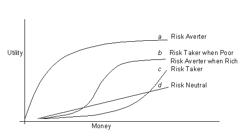
Picture 2.1 ”Different Utility Curves”
Once a person´s utility curve is known, it is possible to replace any monetary value by its utility equivalent for that person.
To construct a utility curve, we need several points (then we draw the curve through these points). For convenience, we find the largest and the smallest monetary value involved in the decision problem and assign utility values of zero and one to these monetary values. Further points of the utility curve can be constructed so that the decision maker visualizes a hypothetical gambling situation and determines the certainty equivalents for various gambles. It is illustrated by the following example.
The extreme outcomes for an entrepreneur
is a loss of $10 million and a gain of $100 million. Suppose that the entrepreneur
considered a hypothetical gambling situation involving two possible outcomes
and found the certainty equivalents for the gambles shown in Table 2.7.
Using these data draw a utility curve.
|
|
|
| 0.5 chance at -10
mil. and
0.5 chance at 100 mil. |
|
| 0.5 chance at 15
mil. and
0.5 chance at 100 mil. |
|
| 0.5 chance at -10
mil. and
0.5 chance at 15 mil. |
|
Table 2.7 ”Certainty Equivalents for Gambles”
The definition of the certainty equivalent results in the following identities.
![]()
![]()
![]()
![]()
![]()
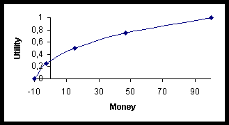
Picture 2.2 ”Utility Curve for the Entrepreneur with Risk Aversion”
The utility curve passes through the following points: [-10;0], [-2.5;0.25], [15;0.5], [47;0.75], [100;1]. It is drawn in Picture 2.2. The curve is concave which indicates that the entrepreneur is risk averter.
There is empirical evidence that the most of decision makers are risk averter (therefore they insure against potential losses). On the other hand, risk preferring individuals exist, too (for example they like to gamble).
2.6.2 Expected Utility Criterion
If we translate the monetary values in a payoff table to their utilities, we can replace the EMV criterion by the expected utility criterion. We calculate the expected utility (EU) for each alternative and choose the alternative with the highest EU.
Refer to Table 2.2, suppose that the grocer expressed
the utilities of the profit values with the numbers shown in Table 3.8.
| Profit |
|
|
|
|
|
|
| Utility |
|
|
|
|
|
|
Table 2.8 “Utility Values of Profit”
If the probabilities of low, moderate, and high demand are 0.3, 0.5, 0.2, respectively, expected utilities of the alternatives have the following values:
EU (small) = 0.9
EU (medium) = 0.3*0.7 + 0.5*0.95 + 0.2*0.95 = 0.875
EU (large) = 0.3*0 + 0.5*0.8 + 0.2*1 = 0.6
The greatest expected utility is connected with the small order and therefore this order should be realized. The same result has been obtained by means of the EMV criterion (see section 2.4) but generally, the best alternatives selected according to the EU and the EMV criterion must not be identical due to the nonlinear relationship between monetary values and their utilities.
2.7 Decision Making with Additional Information
In some situations it is possible to reduce the outcome´s uncertainty and to ascertain which state of nature will actually occur. In these cases, the decision maker doesn´t know whether to decide immediately or delay a decision until it is clear which state of nature will occur. The important question for the decision maker is whether the cost of waiting (e.g., the cost of an option, storage costs) or of additional information (e.g., using marketing research or a better forecasting technique) outweighs the potential gain that more information would permit.
Possible ways of obtaining additional information depend on the nature of the decision problem. For example, information about consumer preferences might come from market research; additional information about a product could come from product testing; legal experts might be called on; and so on.
The value of the additional information
can be quantified by means of the expected value of the perfect information
or the imperfect information.
2.7.1 Expected Value of Perfect Information
The expected value of perfect information (EVPI) represents the increase of the best expected payoff in consequence of obtaining a free, perfect prediction. It can be interpreted as an upper bound on the amount of money the decision maker would be justified in spending to obtain perfect information.
The EVPI is equal to the difference between the expected payoff under certainty (EPC), that is with the perfect information, and the best expected payoff without the perfect information.
The following formulas hold:
EVPI = EPC – max(EMV) for a maximization criterion
EVPI = min(EMV) – EPC for a minimization criterion
There is an important relationship between the EVPI and the EOL. The EVPI is equal to the expected opportunity loss for the best alternative, i. e. to the minimum value of the EOL computed for each alternative. The mentioned relationship can be explained in this way: The perfect information should reduce the opportunity loss that exists under uncertainty due to imperfect information to zero. Hence, the expected opportunity loss of the optimal alternative measures the EVPI and conversely, the EVPI is a measure of opportunities forgone. In this sense, if the EVPI is large, it should be a signal to the decision maker to seek another alternatives.
Refer to Table 2.2, we will determine the EVPI in the grocer´s decision problem.
The best payoff under each state of nature is 50, 52, 54. The probabilities of these states are 0.3, 0.5, 0.2. The expected payoff under certainty is
EPC = 0.3*50 + 0.5*52 + 0.2*54 = 51.8.
The largest expected payoff without the perfect information, as computed in Section 2.4, is
max(EMV) = 50.
Hence,
EVPI = EPC – max(EMV) = 51.8 - 50 = 1.8
The value 1.8 is equal to the lowest expected regret, as computed in Section 2.4.
A useful check on computations is provided by the following identity:
EMV (of any alternative) + EOL (for the same alternative) = EPC
This identity is verified for the grocer´s
problem in Table 2.9. The EMV and the EOL were calculated in Section 2.4.
|
|
|||
|
|
|
|
|
| EMV |
|
|
|
| EOL |
|
|
|
| EPC |
|
|
|
Table 2.9 “Check on Computations of EMV, EOL, EPC”
2.7.2 Expected Value of Sample Information
Most information that we can obtain on states of nature is imperfect in the sense that it doesn´t tell us exactly which event will occur. Even so, imperfect (sample) information will still have value if it will improve the expected profit.
The expected value of sample information (EVSI) represents the increase of the best expected payoff in consequence of obtaining a free imperfect information. It can be interpreted as an upper bound on the amount of money the decision maker is willing to spend to obtain imperfect information.
The EVSI is equal to the difference between the best expected value of payoff with sample information (EVMS) and the best expected value of payoff without sample information.
The following formulas hold:
EVSI = EVMS – max(EMV) for a maximization criterion
EVSI = min(EMV) – EVMS for a minimization criterion
Sometimes it is useful to express the degree of increase in information from a sample relative to perfect information. One way to judge this degree is the ratio of EVSI to EVPI. This is known as the efficiency of sample information (EFSI). This number can range from 0 to 1. The closer the number is to 1, the closer the sample information is to being perfect; the closer the number is to 0, the less the amount of information there is in the sample.
To demonstrate a calculation of the EVSI, we use the following example.
A manager decides about the size of the
future store. His payoffs depend on the size of the store and the strength
of demand. These payoffs (in thousands of dollars) are shown in Table 2.10.
| Demand®
Store |
|
|
| Small |
|
|
| Large |
|
|
Table 2.10 “Payoff Table for Store Planning”
The manager estimates that the probabilities
of low demand and high demand are equal (0.5). These probabilities are
called prior
probabilities. The manager could request that a research firm conducts
a survey (cost $2,000) that would better indicate whether the demand will
be low or high. In discussions with the research firm, the manager has
learned about the reliability of surveys conducted by the firm. This information
is shown in Table 2.11 in the form of conditional
probabilities.
|
|
|
|
|
|
|
|
| Low demand |
|
|
| High demand | 0.1 | 0.7 |
Table 2.11 “Conditional Probabilities of Survey Predictions, Given Actual Demand”
The numbers in Table 2.11 indicate that in past cases when demand actually was low, the survey correctly indicated this information 90 percent of the time, and incorrectly indicated a high demand 10 percent of the time. Moreover, when a high demand existed, the survey incorrectly indicated a low demand 30 percent of the time and correctly 70 percent of the time.
In the further probability calculations we will use these symbols:
event S1 …… low demand
event S2 …… high demand
forecast F1 … information that
the demand will be low
forecast F2 … information that
the demand will be high
The prior probabilities P(S1)
= P(S2) = 0.5 and Table 2.11 contains the conditional
probabilities ![]() .
.
The joint
probability of both a forecast Fj and event Si
is equal to the product ![]() .
These probabilities are shown in Table 2.12. The last column in this table
contains the marginal probabilities of demand level P(Si)
for i = 1,2 (it is the sum of the joint probabilities in each row).
The last row in Table 2.12 contains the marginal
probabilities of survey forecast level P(Fj)
for j= 1,2 (it is the sum of the joint probabilities in each column).
.
These probabilities are shown in Table 2.12. The last column in this table
contains the marginal probabilities of demand level P(Si)
for i = 1,2 (it is the sum of the joint probabilities in each row).
The last row in Table 2.12 contains the marginal
probabilities of survey forecast level P(Fj)
for j= 1,2 (it is the sum of the joint probabilities in each column).
|
|
|
|
|
|
|
|
|
|
| Low |
|
|
|
| High |
|
|
|
|
of Survey Prediction |
|
|
|
Table 2.12 “Joint and Marginal Probabilities Table for Store Planning”
Using the Bayes rule, we can calculate the posterior (revised) probabilities of low and high demand. These values reflect the information from a survey and are given by the following formula:
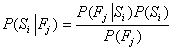 ,
, ![]()
The posterior probabilities based on survey prediction of “low demand” are:
![]()
![]()
If the survey shows “high demand”, the posterior probabilities of low and high demand are:
![]()
![]()
In order to find EVSI, first find the expected
payoffs for small store and large store for these situations: survey shows
“low demand”, survey shows “high demand”, no survey. These calculations
are shown in Table 2.13.
|
|
|
|
|
|
|
|
||
| Small | 0.75*30+0.25*50=35 | 0.125*30+0.875*50=47.5 | 0.5*30+0.5*50=40 |
| Large |
|
|
|
Table 2.13 gives these results:
If the survey shows “low demand” (with the probability 0.6), small store is the best alternative (with the expected payoff $35,000). If the survey shows “high demand” (with the probability 0.4), large store is the best alternative (with the expected payoff $71,250). Hence, the expected payoff for using survey is
EVMS = 0.6*35 + 0.4*71.25 = 49.5
The maximum expected payoff for no survey is max (40;45) = 45. The expected value of sample information is
EVSI = 49.5 - 45 = 4.5 thousand, or $4,500.
Because the EVSI is $4,500, whereas the cost of the survey is $2,000, it would seem reasonable for the manager to use the survey. The expected profit would be $2,500.
If we want to determine the efficiency of the survey in the above mentioned decision problem, we must calculate the expected value of perfect information.
EPC = 0.5*30 + 0.5*80 = 55
max(EMV) = 45
Hence,
EVPI = 55 – 45 = 10,
EFSI = ![]()
The EVSI is always less than the EVPI because the survey can give inconclusive or incorrect information as indicated in Table 2.11.
Taking a sample always represents a means of obtaining only an imperfect information, since the sample is not likely to represent exactly the population from which it is taken.
2.8 Sensitivity Analysis
Analyzing decisions under risk requires working with estimated values of the payoffs and the probabilities for the states of nature. Inaccuracies in these estimates can have an impact on the choice of the best alternative, and ultimately, on the outcome of a decision.
Sensitivity analysis examines the degree to which a decision depends on (is sensitive to) assumptions or estimates of payoffs and probabilities. If this analysis shows that a certain decision will be optimal over a wide range of values, the decision maker can proceed with relative confidence. Conversely, if analysis indicates a low tolerance for errors in estimation, additional efforts to pin down values may be needed.
The aim of sensitivity analysis is to increase the decision maker´s understanding of the problem and to show the effect of different assumptions.
In this section, sensitivity of the choice of the best alternative to probability estimates is examined. The aim of this analysis is to identify a range of probability over which a particular alternative is optimal. The decision maker then need only decide if a probability is within a range, rather than decide on a specific value for the probability of a state of nature.
When there are only two states of nature, a graphical way can be used for sensitivity analysis. A graph provides a visual indication of the range of probability over which the various alternatives are optimal. This procedure is illustrated by the following example.
In the decision problem given in Table 2.14, determine
the ranges for the probability of state #2, for which each alternative
is optimal under the expected value approach (these ranges can easily be
converted into ranges for the probability of state #1).
|
|
|
|
|
|
|
|
|
|
|
|
|
|
|
|
|
|
|
|
Table 2.14 “Payoff Table for Sensitivity Analysis”
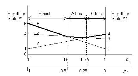
Picture 2.3 ”Graphical Analysis Sensitivity”
The probability range from 0 to 1 can be
depicted on the horizontal axis and the payoffs for each alternative can
be plotted on the vertical axes that are constructed in the points 0 and
1 on the horizontal axis (see Picture 2.3). The payoffs for state #1 are
plotted on the left axis, for state #2 on the right axis. If we connect
the responsive points on both vertical axes, for each alternative we obtain
the graph of the expected value of payoff in dependence on the probability
of state #2 (let´s designate it p2; then p1
= 1 – p2). The
equations of the expected value lines can be easily derived.
The graphical sensitivity analysis requires all the expected value lines to be plotted on the same graph. The highest line for any given value of p2 represents the optimal alternative for that probability (it is the heavy line on Picture 2.3). Thus, referring to Picture 2.3, for low values of p2 (and thus high values of p1), alternative B will have the highest expected value; for intermediate values of p2, alternative A is best; and for higher values of p2, alternative C is best.
If we want to ascertain these ranges of
probability exactly, we need to determine where the upper parts of the
lines intersect. It is an algebraical problem: to solve together two equations
that represent the respective lines. These equations have the form y
= a + bx, where a is the y-intercept value at the left
axis, b is the slope of the line, and x is p2.
Because the distance between the two vertical axes is 1, the slope of each
line is equal to the difference of payoffs under state #1 and state #2
for the respective alternatives. The slopes and equations of the lines
are shown in Table 2.15.
|
|
|
|
|
|
|
|
|
|
|
|
|
|
|
|
Table 2.15 “Equations of the Expected Value Lines”
To determine the intersections of the lines that belong to the alternatives A, B, C, we set the right-hand-sides of the respective equations equal to each other and solve for p2.
|
|
|
|
|
|
|
|
|
|
|
|
|
|
|
Table 2.16 “Calculation of Intersections of Expected Value Lines”
The results of the above sensitivity analysis are
summarized in Table 2.17.
|
|
|
|
| A is optimal |
|
|
| B is optimal |
|
|
| C is optimal |
|
|
At the intersection of the lines that represent the expected values of the alternatives, the two alternatives are equivalent in terms of expected value. Hence, the decision maker would be indifferent between the two alternatives at these points.
A graphical sensitivity analysis can be
used also for a minimization criterion. The graph is equal as for a maximization
criterion. However, the smallest expected value of the criterion is plotted
by the lowest parts of the lines that represent expected values of the
alternatives.