5.1. Introduction
Multiple criteria decision-making (MCDM) refers
to making decisions in the presence of multiple - usually conflicting criteria.
Problems for multiple criteria decision making are common occurrences in
everyday life and many examples can be found.
Examples
of MCDM
Decision is understood as choice of one variant
from certain list of real possible variants. This chosen variant is considered
to be optimal but often designation what is optimal is the most difficult
part of problem. We have to take in mind that many criteria are contradictory
and interests of various subject of decision making can be in conflict
(shop owner x customer). Even one person cannot some times make his/her
decision without inner conflict.
Another problem is quantification of available information.
Some input information are quantitative (price of new shoes – we get precise
number expressed in money units) and some kinds of information are not
directly quantitative and must be transferred into numbers (beauty, modishness,
durability etc.) There are many methods for doing that but each has advantages
and disadvantages and certain influence of subjective opinion is not excluded.
Example:
School Grades
Belief in quantitative data generally depends on
local tradition and type of solved problem. Many people still prefer intuition
and experience. The true is that there are no methods (and never will be)
for algorithmisation of whole decision process but using quantitative methods
can lay aside big mistakes (dominated variants – see latter).
The theory on mathematical modelling, but some parts
don’t require deep mathematical knowledge and could be study independently.
Especially exploitation of some software is simple. On the other hand deeper
knowledge of MCDM methods including mathematical background leads to more
serious access and better interpretation of results. This text contains
classification of MCDM methods, characteristic of each class of methods.
Detail description is supplemented only to several best known and widely
used methods.
The aim of studying this text is not to be familiar
with each existing method (impossible due to high number of methods and
continual development of new), but understanding of basic principles and
ability to use some methods (via software) and explain results.
5.2. Basic Concepts
All MCDM problems have the following common characteristics:
Multiple objectives/attributes
Each problem has multiple objectives/ attributes.
A decision-maker must generate relevant objectives/attributes for each
problem setting.
Conflict among criteria
Multiple criteria usually conflict with each other
(for example the quality and price of goods).
Incommensurable units
Each objective/attribute has a different unit of
measurement. In the car selection case, gas mileage is expressed by miles
per gallon (MFG), comfort is by cu ft if fit is measured by passenger space,
safety may be indicated in a nonnumeric way, cost is indicated by dollars,
etc.
Design/selection
Solutions to these roblems are either to design
the best alternative or to select the best one among previously specified
finite alternatives.
There exist two alternative sets due to the different
problem settings: one set contains a finite number of elements (alternatives),
and the other has an infinite number.
The problems of MCDM can be broadly classified into
two categories in this respect:
Multiple Attribute Decision Making - MODM (in
this chapter)
Multiple Objective Decision Making – MADM (in
following chapter)
Multiple objective decision-making (MODM) is not associated with the problem where the alternatives are predetermined. The thrust of these models is to design the 'best' alternative by considering the various interactions within the design constraints which best satisfy the decision maker by way of attaining some acceptable levels of a set of some quantifiable objectives.
The common characteristics of MODM methods are that
they possess:
1) a set of quantifiable objectives
2) a set of well defined constraints
3) a process of obtaining some trade-off information,
implicit or explicit, between the stated quantifiable objectives and also
between stated or unstated nonquantifiable objectives.
MODM is associated with design problems (in contrast
to selection problems for the MADM).
In MADM, there are usually a limited (and countable) number of predetermined alternatives. The alternatives have associated with them a level of the achievement of the attributes (which may not necessarily be quantifiable) based on which the final decision is to be made. The final selection of the alternative is made with the help of inter- and intra-attribute comparisons. The comparisons may involve explicit or implicit trade-off.
5.2.1. Terms and Definitions
Criteria -
A criterion is a measure of effectiveness, basis for evaluation.
Goals – A priori values or levels
of aspiration. These are to be either achieved or surpassed or not exceeded.
Attributes – Each alternative can
be characterised by a number of attributes = characteristics = parameters
= factors = properties.
Objectives - Something to be pursued
to its fullest, generally direction of planned change. For example the
farmer wants to maximise his profit or minimise production costs or minimise
the water pollution.
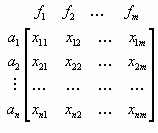
Decision matrix – The MADM problem
can be expressed in a matrix containing criteria in columns and variants
in lines. Elements xij indicate evaluation of alternative i
with respect to criterion j.
Hence variant ai, i= 1,2,...m
Is denoted by line vector
xi=(xi1,xi2,…,xin)
and column vector
xj=(x1j,x2j,…,xmj)
shows the contrast of each alternative
with respect to attribute fj.

Example:Washing
machines - Decision Matrix
Transformation to All Maximal Criteria
-
Many MADM methods suppose that all criteria are maximising. To be in line
with this demand we must transfer minimising criteria to maximising. For
example minimising criterion ”Price” we can transfer to maximising criterion
”Saved money”. The most expensive variant will have zero in the ”Saved
money” column and other – cheaper variants – the value one can save comparing
with the most expensive variant.
Example:
Washing Machines – Criteria Transformation
Dominated variant – Variant ![]() is dominating variant
is dominating variant
![]() (dominated variant) if
(dominated variant) if
5.2.2. Normalisation
A normalisation may be essential for some
methods to facilitate the computational problems inherent to the presence
of different units in decision matrix. The advantage of normalisation is
that all criteria are measured in dimensionless units and inter-attribute
comparison is possible. The normalisation procedure doesn’t lead to equal
minimum and maximum values for all attributes, so straightforward comparison
is still difficult.
There are different methods of normalisation,
some of then will be mentioned together with particular MADM method.
Vector normalisation
This procedure implies that each row in
decision matrix is divided by its norm. The elements of normalised matrix
R are calculated:

![]()
5.2.3. Weights Assessing
Many methods require information about the relative importance of each attribute (or objective). It is usually given by a set of (preference) weights, which is normalised to sum to 1. In case of n criteria, a set of weights is

Sequence Method
The decision-maker should be able to arrange criteria
according their importance to a sequence from most to least important.
A natural numbers from k to 1 are assigned to criteria (most important
criterion number k, second most important k-1 etc.). The weights are calculated
as follows:
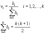
Sum of bi is equal to sum of first k natural numbers
Saaty’s Matrix
The decision-maker is supposed to judge the relative importance of each pair of criteria. The elements of matrix are considered to be an estimation of importance of i-th and j-th criteria. The scale 1,3,5,7,9 is often used.
Verbal Explanation of the Scale
![]()

The estimations of weights are designated by minimisation of the quadratic form:
![]()
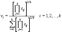
LINMAP
LINMAP (Linear Programming Techniques for Multidimensional
Analysis of Preference) is a method for assessing the weights of attributes
as well as for selecting the alternative.
LINMAP
5.3. Methods for Multiple Attribute Decision Making
5.3.1. Classification of MADM Methods
The available input information varies. One may not indicate his preferences at all, or may represent his preference through the form of attribute or alternative. The degree of judgement skill also varies. For instance, we may list the different preference information on attributes by the ascending order of complexity: standard level, ordinal, cardinal, and marginal rate of substitution.
We classify methods for MADM based upon different forms of preference information from a decision-maker.
1. Class – Methods of No Information Given
Dominance
Maximin
Maximax
2. Class – Methods for Information on Attribute
Given
2.1. Methods for Standard level of Attribute
Given
Disjunctive Method
Conjunctive Method
2.2 Methods for Ordinal of Attribute Given
Lexicographic Method
Elimination by Aspects
Permutation Method
2.3 Methods for Cardinal Information of Attribute
Given
Linear Assignment method
Simple Additive Weighting Method
Hierarchical Additive Weighting Method
ELECTRE
TOPSIS
2.4 Methods for Marginal Rate of Substitution
of Attribute Given
Hierarchical Trade-offs Method
3. Class - Methods for Information on Alternative Given
3.1 Methods for Pairwise Preference Information
Given
LINMAP
Interactive Simple Additive Weighting Method
3.2 Method for Order of Pairwise Proximity Information
Given
Overview
of MADM Methods
Description of some of these methods follows.
If there is no information on criteria importance
we have to use one of the method of 5.4 chapter.
If preference information either on attributes or
alternatives is available, the information can be expressed in various
ways:
1) standard level of each attribute (chapter 5.5)
2) relative importance by ordinal preference (chapter
5.6)
3) relative importance by cardinal preference (chapter
5.7)
4) marginal rate of substitution between attributes
5.4. Methods without Preference Information
5.4.1. Dominance
An alternative is dominated if there is another alternative, which excels it in one or more attributes and equals it in the remainder. Eliminating the dominated ones can reduce the number of alternatives. A set of nondominated solutions is one obtained through the sieve of dominance method. There are no assumptions so we don’t need to transfer minimising criteria to maximising. Steps of the method:
5.4.2. Maximin
Under this procedure only a single weakest attribute represents an alternative; all other (n-1) attributes for a particular alternative are ignored. If these lowest attribute values come from different attributes, as they often do, we may be basing our final choice on single values of attributes that differ from alternative to alternative. Therefore, the maximin method can be used only when interattribute values are comparable; that is, all attributes most be measured on a common scale; however, they need not be numerical.
The alternative, A +, is selected such that:

5.4.3. Maximax
The maximax method selects an alternative by its best attribute value. In this case the highest attribute value for each alternative is identified and these maximal value are compared. The alternative with highest such value is to be chosen. All criteria must be measured in the same scale, if not use (5.13) or more complicated formula (5.3) or other formulas designed for criteria transformation.
The alternative, A +, is selected such
that:
![]()
5.5. Methods for Standard Level of Attribute Given
The decision-maker sets the minimal attribute values (standard levels) he/she will accept for each attribute. Any alternative that has an attribute value less than standard level will be rejected (is not acceptable). This procedure is called conjunctive method. If the variant is accepted in the case at least one attribute is over or equal to standard level the method is called disjunctive.
5.5.1. Conjunctive Method
We classify Ai as an acceptable variant only if
We classify Ai as an acceptable alternative only if:
The most important information needed is the ordinal interattribute preference information. The relative importance among attributes determined by ordinal preference is less demanding for the decision-maker to assess than by cardinal preference.
5.6.1. Lexicographic Method
In some decision situations a single attribute seems to predominate. One way of treating this situation is to compare the alternatives on the most important attribute. If one alternative has a higher attribute value than any of the other alternatives, the alternative is chosen and the decision process ends.
However, if some alternatives are tied on the most important attribute, the subset of tied alternatives are then compared on the next most important attribute. The process continues sequentially until a single alternative is chosen or until all n attributes have been considered.
5.6.2. Permutation Method
The method consists of testing each possible ranking of the alternatives against all others. With m alternatives, m! permutation rankings are available, so it is not convenient for big models. The method will identify the best ordering of the alternative rankings, then the dominating alternative. The method can be used also if the cardinal preferences are known.
If there are only ordinal preferences we can define cardinal preferences using for example Sequence Method (see chapter 5.2.3).
Case of cardinal preferences
Suppose a number
of alternatives A1,…,Am have to be evaluated according
to a attributes f1,…fn. Assume that a set of cardinal
weights v1,…,vn be given.
Let’s have three
alternatives: A1, A2, and A3. Then six permutations of the ranking of the
alternatives exist (m! = 3! = 6). They are:
P1=A1,A2,A3 P3=A2,A1,A3 P5=A3,A1,A2
P2=A1,A3,A2 P4=A2,A3,A1 P6=A3,A2,A1
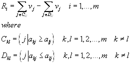
For each permutation
we compare all pairs of variants. If in the partial ranking of variants
Ak and Al under j-th criterion is ![]() we
put the criterion weight vj into set Ckl, if
we
put the criterion weight vj into set Ckl, if ![]() we
are put the vj to the set Dkl.
we
are put the vj to the set Dkl.
Then the evaluation
criterion of permutation Pi is given by:
Example:Fighter
Aircraft Problem – Permutation Method
5.7. Methods for Cardinal Preference of Attributes
The methods in this class require the cardinal preferences of attributes. This (a set of weights for the attributes) is the most common way of expressing the interattribute preference information.
5.7.1. Linear Assignment Method
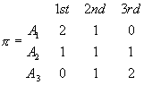
The linear assignment method is based on a set of attribute-wise rankings and a set of attribute weights. The method features a linear compensatory process for attribute interaction and combination. In the process only ordinal data, rather than cardinal data, are used as the input. This information requirement is attractive in that we do not need to scale the qualitative attributes.
The method is to
pick the sum of ranks for each alternative and rank them from the lowest
sum to the highest sum. For instance, consider the following attributewise
preferences with equal weight:
|
|
|||
|
|
|
|
|
|
|
|
|
|
|
|
|
|
|
|
|
|
|
|

5.7.2. Simple Additive Weighting Method
Simple Additive Method
(SAW) is probably more often used method of MADM.
The method is based
on maximal the trade-off of variants. The simplification is established
by considering only linear function of trade-off.
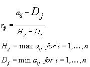
The method requires
all maximal criteria, the same scale for and existing weights’ vectors.
Multiplying the
scale rating for each attribute value by importance weight assigned to
the criterion and then assuming these products over all criteria obtain
total trade-off u (ai) for each alternative.
![]()
5.7.3. TOPSIS
(Technique for Order Preference by Similarity to Ideal Solution)
TOPSIS takes the cardinal preference information on attributes. The ideal solution is guaranteed to have the longest distance to the negative ideal solution.
TOPSIS assumes that each attribute in the decision matrix takes either monotonically increasing or monotonically decreasing utility. In other words, the larger the attribute outcomes, the greater the preference for the "benefit" criteria and the less the preference for the "cost" criteria. Further, any outcome, which is expressed in a nonnumeric way should be quantified through the appropriate scaling technique. Since all criteria cannot be assumed to be of equal importance, the method receives a set of weights from the decision-maker.
The proposed method will be presented in steps:
(Assumption: All maximal criteria see 5.1.1)
Step 1. Construct
the normalised decision matrix
This process tries
to transform the various attribute dimensions into non-dimensional attributes,
which allows comparison across the attributes. An element rij
of the normalised decision matrix R can be calculated as:

Step 2. Construct
the weighted normalised decision matrix
This matrix can
be calculated by multiplying each column of the matrix R with its associated
weight vj. Therefore, the weighted normalised decision matrix
W is equal to:

![]()


![]()

Step 6. Rank the Preference
Order
The variant that is closest
( ciclose to 0) to the negative ideal variant has the highest
distance from ideal variant and is taken as worst variant. Variant with
highest distance from negative ideal variant (ci close to 1)
is closest to ideal variant and can be chosen as best.

A set of alternatives can now be ranked according to descending order of ci.
Example:Washing Machines – TOPSIS
5.7.4. Electre
(Elimination et Choice Translating Reality)
ELECTRE uses the
concept of an 'outranking relationship'. The outranking relationship of ![]() says
that even though two alternatives k and l do not dominate each other mathematically,
the decision maker accepts the risk of regarding Ak as almost
surely better than Al.
says
that even though two alternatives k and l do not dominate each other mathematically,
the decision maker accepts the risk of regarding Ak as almost
surely better than Al.
This method consists of a pairwise comparison of alternatives based on the degree to which evaluations of the alternatives and the preference weights confirm or contradict the pairwise dominance relationships between alternatives. It examines both the degree to which the preference weights are in agreement with pairwise dominance relationships and the degree to which weighted evaluations differ from each other. These stages are based on a 'concordance and discordance' set; hence this method is also called concordance analysis.
The ELECTRE method takes the following steps:
Step 1. Calculate the normalised decision matrix –see (5.21) TOPSIS
Step 2. Calculate the weighted normalised decision matrix – see (5.22) TOPSIS
Step 3. Determine
the concordance and discordance set
For each pair of
alternatives the set of decision criteria is divided into two distinct
subsets. The concordance set Ckl for Ak and
Al is composed of all criteria for which Ak is preferred
to Al. The complementary subset is called discordance set.
Step 4. Calculate
the concordance matrix
The relative value
of the concordance set is measured by concordance index, which is
equal to the sum of weights associated with criteria contained in the set.
The concordance index for normalised weight set is:
![]()
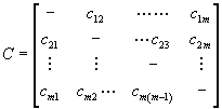
The
successive values of concordance idices ckl (k,l = 1,2,…,m;
k? l) form the concordance matrix C (m x m):
Step 5. Calculate
the discordance matrix
The concordance
index reflects the relative dominance of a certain alternative over a competing
alternative on the basis of the relative weight attached to the successive
decision criteria. So far no attention has been paid to the degree to which
the evaluations of a certain Ak are worse than the evaluations
of competing AR. Therefore a second index, called the discordance index,
has to be defined:

Higher value of dkl implies that, for discordance criteria (=criteria preferring Al) , Al is more favourable that Ak; lower value of dkl Al is less favourable than Ak.
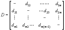
The discordance idices
form the discordance matrix D (m x m):
Step 6. Determine
the concordance dominance matrix
Ak will
only have a chance of dominating Al , if its corresponding concordance
index ckl exceeds at least a certain threshold value i.e. ![]() .
.
The threshold value can be determined as:

![]()
Step 7. Determine
the discordance dominance matrix
This matrix is constructed
in a way analogous to the F matrix on the basis of a threshold value d
to the discordance indices. The elements of gkl of the discordance
dominance matrix G are calculated as:
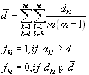
Also the unit
elements in the G matrix represent the dominance relationships between
any two alternatives.
Step 8. Determine
the aggregate dominance matrix
The next step is
to calculate the intersection of the concordance dominance matrix F and
discordance dominance matrix G. The resulting matrix, called the aggregate
dominance matrix E, is defined by means of its typical elements ekl
as:
![]()
Step 9. Eliminate the
less favourable alternatives
The aggregate dominance matrix
E gives the partial-preference ordering of the alternatives. If ekl
= 1, then Ak is preferred to Al for both the concordance
and discordance criteria, but Ak still has the chance of being dominated
by the other alternatives. Hence the condition that Ak is not
dominated by ELECTRE procedure is:
![]()
This
condition appears difficult to apply, but the dominated alternatives can
be easily identified in the E matrix. If any column of the E matrix has
at least one element of 1, then this column is 'ELECTREcally' dominated
by the corresponding row(s). Hence we simply eliminate any column(s) which
have an element of 1.
Example: The Fighter Aircraft Problem – ELECTRE
Bibliography:
Ching-Lai Hwang, Kwangsun
Yoon: Multiple Attribute Decisin Making, Springer Verlang Berlin Heidelberg
New York 1981
Fiala P.,Jablonský J., Maňas
M.: Vícekriteriální rozhodování,VŠE Praha 1997
Šubrt T. a kol.: Ekonomicko
matematické metody II, Aplikace a cvičení , ČZU Praha 2000