8.1 The Terminology of Network Models
 

Network models have mathematical structures that are effectively exploited. We discuss the general mathematical structure of network models now. Later in this sections, we discuss some special network problems.

Planning the distribution of products, planning the building of a house or planning the sewerage or drainage system are common application for network models. Let's think of network models for physical distribution of grain as we describe network models in general. This kind of model will be used to illustrate the terminology of network models.

A network model consists of nodes connected by arcs. Think of nodes as cities and arcs as roads and of a network as consisting of cities connected by roads. A directed arc has a direction associated with it. For example, traffic goes in only one direction on a one-way road.

Picture 8.1 ”Example of Network”

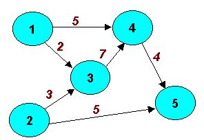
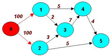
Picture 8.1 illustrates an example with 7 nodes and 10 directed arcs. The arc directions are indicated by the arrows. For each road, a cost for use and a maximum capacity limit can be imposed.

 

Picture 8.2 ”Example of Network with Nodes Numbered”

Picture 8.2 has the network of Picture 8.1 with the nodes numbered 1 through 7. In this example, the arc connecting Node 5 to Node 6 is called Arc (5,6). The first number is assigned to the node at the beginning of the arc, and the second number is assigned to the node at the end of the arc (arrow). Doing this specifies the direction of the arc. The cost per unit shipped from Node i to Node j, the maximum capacity from Node i to Node j and anet stock position of each node can be specified. (For more information see Node positions and arc capacities in networks.)

A network model is defined by specifying the nodes and their net stock positions, and the arcs and their costs, minimums, and maximum capacities. We call a pictorial representation such as Picture 8.2 the network model. Such a picture helps us understand the network.

There are many special network problems. These problems are special cases of the general network model. Some of them have additional restrictions on how nodes are connected. Some don't have capacity limits. Some have different assumptions on the initial amounts on hand or the amounts to be dropped off at nodes.

Before we discuss special network problems, let's state an important property of optimal, corner point solutions for general network problems. For each of the network models discussed, if the net stock positions, minimums, and capacities are integer values, all corner point solutions result in every variable value being integer. Because the simplex method gives an optimal corner point solution, this method and its variants achieve optimal solutions with integer variable values.

We discuss each special network problem in a separate section. For each, we describe applications, and discuss the mathematical structure.

8.2 The Maximum Flow Problem
 

Let's consider a network that has one input node and one output node. The maximum flow problem finds the maximum flow from the input node to the output node. The arcs have flow capacities.

In one application of this problem, a water station company analyzes a water pipeline system used to transport drinking water from the main water station to surrounding cities and villages. The capacity of a water pipeline segment depends on its diameter and the pumping stations and tank towers. The company wants to determine the maximum flow of the pipeline system in order to plan for peak consumption during the day.

In another application, a long-distance telephone company uses the maximum flow problem to determine the maximum number of simultaneous calls that can be made between two cities. Phone calls can be routed in many ways between them. Lines between pairs of cities along the routes have different capacities.

Let's consider an Aqueduct Problem. One section of the aqueduct must be completely closed due to a general repair. When the section is closed, several ”pipeline detour” are available. Let's develop a maximum flow problem to determine the maximum flow that the alternate section can handle.

The possible water pipeline detours are illustrated in Picture 8.3. The arcs are pipelines between different points - water tanks, reservoirs or pumping stations. Nodes 1 and 8 are points on the closed section. Node 1 is the beginning of the planned section closing, and Node 8 is the end of it.

The number on each arc is the water capacity of the pipeline in cubic meters (m³) per minute. The 2 on Arc (2,4) indicates that 2 m³ of water is the maximum flow on the pipe from Node 2 to Node 3. The flows between the nodes are only in one direction. Let's find the maximum flow from Node 1 to Node 8.

If the maximum flow is large enough, the inhabitants, water-house clients, will not be limited by the section closing.

Our problem has its own algebraic representation and can be described using maximum flow problem mathematical model and solved using simplex method. The optimal solution provided by Linkosa software (see SW download) is shown in Table 8.1. Structure of the model inputs for Linkosa Solver is available here. Such problem could be well solved using LINDO.

 

Optimal Solution of the Model Aqueduct
Max. value of the objective function Max Flow is 11
Structural variables				Constraints
Name	Value	Type		Name	Value	Slack
Z	11	Basic		Node 1	0	0
X1,2	5	Basic		Node 2	0	0
X1,3	6	Upper bound		Node 3	0	0
X2,4	2	Upper bound		Node 4	0	0
X2,5	3	Basic		Node 5	0	0
X3,4	1	Basic		Node 6	0	0
X3,6	5	Upper bound		Node 7	0	0
X4,5	3	Basic		Node 8	0	0
X5,6	4	Upper bound
X5,7	2	Basic
X6,7	2	Basic
X6,8	7	Upper bound
X7,8	4	Upper bound

The maximum flow is 11, or 11 m³ of water per minute. The solution shows the amount of water per minute for each pipeline in the alternate system. For example, 3 m³ of water per minute will flow from Node 4 to Node 5 (variable x_4,5), 4 m³ of water per minute will flow from Node 7 to Node 8 (variable x_7,8).

8.2.1 More then One Input or Output Node

We discussed the maximum flow problem with only one input node and only one output node. Let's consider an example with two input nodes. In Picture 8.3. the output node is Node 5, but Nodes 1 and 2 are both input nodes. We want to find the total maximum flow from Nodes 1 and 2 to Node 5.

Picture 8.4 "Maximum flow Example with Two Starting Nodes"

The easiest solution of such problem is to modify the network model so that it has only one input node. We introduce a dummy node - Node 0 and arcs from Node 0 to all of the input nodes. In this example, you introduce arcs to Nodes 1 and 2 as illustrated in Picture 8.4. The capacities on Arcs (0,1) and (0,2) are infinite. For practical solutions they will be very high (”high enough”), much higher than the highest arc capacity in the model – for example 100.

 
 

Picture 8.5 "Network Model with Dummy Starting Node Added"

This transformation allows solving a maximum flow problem with two sources by maximum flow software that requires only one input node and one output node. If there is more than one output node, use a similar modification by creating a dummy node that follows all of the possible output nodes to the dummy output node.

8.3 The Shortest Route Problem

The shortest-route problem is a network problem with many applications. As an example, say that you are planning to fly to Singapore for a vacation from the starting point in Prague. You examine a world map to select the route. Suppose that you minimize the distance and not the flying ticket price (it usually does’nt depend on the distance so closely). The world map shows cites (nodes) connected by airlines (arcs) and the distances on each route - line connecting a pair of cities. The total distance for a route is obtained by adding all of the distances on that route. Your objective is to find the route to Singapore, with the smallest total distance. Thus, your problem is a shortest-route problem.

For this shortest-route problem, each arc has a numerical value (distance in kilometers) but those numbers do not always have to signify distances, they can signify costs as well. You want to pick the route that minimizes the sum of the numbers on the arcs.

Picture 8.6 shows possible flight segments from Prague to Singapore. The distance between each two cities are on the arcs, the node numbers are small red numbers nearby the nodes. You want to minimize the total distance from Prague to Singapore. The nodes are the airports, and the arcs are the flights. You define the net stock position as + 1 at Prague and - 1 at Singapore. The net stock positions at other nodes (airports) are 0. The model has a decision variable, x_ij, for each arc. Because the net stock positions are + 1 , 0, and - 1, the x_ij , must be <= 1. As with many network models, the optimal corner point solution has integer variable values. Thus, the x_ij, are all 0 or 1 (Boolean). If x_ij = 1, the arc is included in the shortest route; if x_ij = 0, the arc is not included. be limited by the section closing.

This problem has the algebraic representation similar to maximum flow problem and can be described using bivalent programming mathematical model.

 
The optimal solution provided by Linkosa software (see SW download) is shown in Table 8.1.
 

Optimal Solution of the Model Shortest Route
Min. value of the objective function Distance is 10560
Structural variables				Constraints
Name	Value	Type		Name	Value	Slack
X1,2	0	Lower bound		Prague	1	0
X1,3	1	Basic		Frankfurt	0	0
X1,4	0	Lower bound		Vienna	0	0
X2,6	0	Basic		Zurich	0	0
X3,5	1	Basic		Amman	0	0
X4,5	0	Lower bound		Dubai	0	0
X4,8	0	Basic		Bombay	0	0
X5,6	1	Basic		Bangkok	0	0
X5,8	0	Lower bound		Singapore	1	0
X6,7	0	Lower bound
X6,9	1	Basic
X7,8	0	Basic
X8,9	0	Basic

The shortest route consist of flight segments Prague – Vienna (x_1,3 = 1), Vienna – Amman (x_3,5 = 1), Amman – Dubai (x_5,6 = 1) and Dubai – Singapore (x_6,9 = 1). The sum of these flight segments length generates the minimum total distance from Prague to Singapore, 10560 km.

You can find the shortest route from Prague to Singapore by careful examination of the network too. List all of the possible routes and total the flight distance on each route. Then, pick the shortest route. However, for shortest-route problems with many nodes and arcs, you need a computer.

lf you must solve many shortest-route problems through a complex network, you can use shortest-route software that is more efficient than LINDO or Linkosa software. But except for networks with a very large number of nodes and arcs, it is generally not necessary to search for software that uses the most efficient algorithm for your shortest-route

If you have complex shortest-route problems, you should understand two important factors in selecting software-the variety of the problem and the network structure.

The variety is the set of nodes for which you need the shortest route. For example, do you just want the shortest route between one pair of nodes-Prague and Singapore? Or do you want the shortest route from one node to all other nodes? It is possible to use an algorithm for the first variety of problem to solve all of the other varieties. You do this by repeating the algorithm for each desired pair of nodes. However, because this procedure repeats many calculations, it is inefficient.

The other factor is the network structure. You should understand the distinction between cyclic networks and acyclic networks. If your network is acyclic, software using an acyclic network algorithm is more efficient than software using a cyclic network algorithm. Acyclic networks are much easier to analyze than cyclic networks. Thus, algorithms for acyclic networks are much more efficient then algorithms for cyclic networks.

8.4 The Critical Path Methods and Project Management

You can use management science for planning, scheduling, and controlling complex projects consisting of many separate activities. For a simple project, you can plan, schedule, and control the activities without a computer. But if a project is very complex, using your mind to keep track of the plan and monitor the progress is difficult. To plan, schedule, and control such projects, you can use the Critical Path Method (CPM) or Metra Potential Method (MPM) for deterministic projects and Project Evaluation and Review Technique (PERT) for stochastic projects. Some advanced methods for project management such as Critical Chain (CCM) or Q-GERT will not be mentioned in this chapter.

Common applications of these methods include:

1. Major construction projects applications
2. Research and development projects
3. Maintenance of complex equipment

There are many successful applications of all these methods in project management in civil engineering, marketing and business development, software development, reingeneering, program management and control and so on.

To complete such projects as on time, you must schedule various activities (tasks). The interdependencies of the activities makes the coordination complicated. Some activities must be completed before others begin, and some activities require the same resources, so you must allocate the resources among them.

As the project manager, you want to know the answers to four questions:

1. What is the goal of the project - can I define its finish (start)?
2. How long will the project take - when it ends (starts)?
3. What tasks are critical? That is, which tasks must be completed on time so that completion of the project is not delayed?
4. Which tasks can be delayed? What will happen delaying them?
5. Do I have enough resources for project realization?
6. Do I have enough money for project realization?
7. Can I minimize the project total cost? - How ?
8. Can I minimize the project duration? - How ?

PERT was developed to manage the Polaris missile project in the 1950s. Because the time for completing activities was uncertain, PERT included probabilistic activity times. CPM was developed for major preventive maintenance projects at Du Pont. Because cost was a major consideration in these programs, CPM included costs. MPM method was developed in France in 1958 to be able to create and calculate projects with various types of dependencies between tasks, when the start of successor task doesn’t depend on the finish of a predecessor task.

8.4.1 Constructing the Project Network

To analyze a project, you must list the activities required to complete the project. For each activity, you list its immediate predecessors and its estimated time. (Later, we discuss probabilistic activity times.) A precedence requirement specifies that an activity must be completed before another is begun (Later, we discuss another possibility for MPM models).You can use a network to describe a project. A network consists of nodes and arcs connecting them. There are two approaches to representing a project by a network. The activities on arcs (AOA) approach where activities on arcs represents an activity as an arc, and the activities on nodes (AON) approach represents an activity as a node (MPM method). At first, we use the AOA approach.
 

Table 8.1 lists the tasks and their immediate predecessors for the project ”Building of a House”. Tasks ”Site Plan” and ”Building Plan” have no predecessors, so it can begin immediately. However, all other tasks can’t start until their predecessors have been completed.

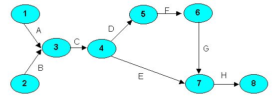
Let's construct the AON network for the this project. We use the arrows on the arcs to show relationships between tasks. Picture 8.1shows one part of a network model for ”Building of a House” Project. Each node represents an event, the starting or finishing of an activity. Nodes 1 (Site Plan) and 2 (Building Plan) are both the project starting events. Node 3 (Construction Permit and Contract) is the event at which Tasks 1 and 2 are finished.

To construct an AON network is much easier then to construct an AOA one.

Picture 8.7 ”AON Network Model for the Table 8.1 Project (Output from Microsoft Project ®)”

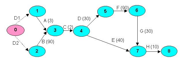
Picture 8.8 "AOA Network Model for the Table 8.1 Project"

8.4.2 Finding the Critical Path
 
 

Say that you're responsible for the project described in Table 8.1. Your costumer wants to have the house completed as soon as possible, and he wants to know the expected completion time for the construction. Sometimes you can work only on one task and sometimes, it's possible to work on more than one activity at a time. For example, you can prepare site plans and building plans at the same time. Picture 8.1

shows the AON network model and Picture 8.3 the AOA model. Let’s calculate the AOA model . Nodes 0 and 9 represent starting and finishing the project, respectively.

For this simple network, we can find the completion time by inspection. There are four paths from Node 1 to Node 6.

1. The path D1-A-C-D-F-G-H totals 0 + 3 + 2 + 30 +90 + 30 +10 = 165 days.
2. The path D2-B-C-D-F-G-H totals 0 + 90 + 2 + 30 +90 + 30 +10 = 252 days.
3. The path D1-A-C-E-H totals 0 + 3 + 2 + 40 + 10 = 55 days.
4. The path D2-B-C-E-H totals 0 + 90 + 2 + 40 + 10 = 142 days.

The critical path is the longest path through the network. For our project critical activities, the critical path is B-C-D-F-G-H with a duration of 252 days. The critical activities are on the critical path. Delaying the completion of a critical activity delays completion of the project. The critical activities are B, C, D, F, G and H. For example, if Activity G takes 35 days rather than 30, the project completion time increases to 257 days.

You can find the critical path by solving a longest-route problem (modification of the mathematical model of shortest route problem). We discussed solving the shortest-route problem by linear programming optimization model. You give the starting node a net stock position of + 1 and the finishing node a net stock position of - 1. For minimization software, let the arc costs be the negative of the activity times. You can also use special, shortest-route software.

Now let's discuss the widely used method of finding the critical path through a network - the CPM.

The classical CPM uses the forward and backward pass calculations for finding the critical path. For the house building project, we've answered two of the four questions. The project can be completed in 252 days, and Activities B, C, D, F, G and H are critical. If the network is simple, you can answer the first two questions by listing all of the possible paths and finding the longest. But for complex networks, this is very complicated and time consuming. Also, we still need to answer the other two questions: What are the starting and finishing times for each activity, and how long can noncritical activities be delayed without delaying project completion? We show how to answer all four questions by the forward and backward pass calculations.

For all CPM calculations, note that the network is acyclic. Every project management network is acyclic, and this simplifies finding the longest (or shortest) path. The earliest start time is the earliest an activity can start, and the earliest finish time is the earliest it can finish. The latest start time is the latest an activity must start, and the latest finish time is the latest it must finish. The procedure for finding critical path has 8 steps, which can be described using CPM algebraic representation , and at the end of it we can answer all the questions mentioned above. Critical activities have the total slack equal to zero, noncritical activities have the total slack greater then zero. The total slack for noncritical activity shows, how the activity can be delayed without delaying project completion.

Besides the basic CPM calculations a more precise analysis of activity slacks can be done.
 

Kind of a slack	Meaning of a slack
Total	How the activity can be delayed without delaying project completion.
Free	How the activity can be delayed without delaying a next task (successor activity).
Independent	How the activity can be delayed without delaying a next task (successor activity) considering the latest realization of its start node.
Dependent	How the activity can be delayed without delaying project completion considering the latest realization of its start node.

All the slacks can be displayed graphically on a timescale.

Let’s have the project described in Table 8.1 and its AOA model representation (Picture 8.3). Table 8.1 summarize the forward pass procedure (earliest starts and earliest finishes of all activities are calculated).

• First set E₀ =0 (Event 0 or Node 0 earliest realization) because dummy activities have no predecessors, it starts at Time 0.
• If Activity D1 starts at 0 and takes 0 days, its earliest finish time is 0 days. The only activity before Node 1 is D1 (0,1), so E₁ = 0.
• If Activity D2 starts at 0 and takes 0 days, its earliest finish time is 0 days. The only activity before Node 2 is D1 (0,2), so E₂ = 0.
• Activity A (B) can start only after Event 1 (2), so their earliest start times are 0.
• The earliest finish time for activity A is its start time plus its duration (0+3=3).
• The earliest finish time for activity B is its start time plus its duration (0+90=90).
• Event 3 has both A and B predecessors, so E₃ = maximum (3,90) = 90.
• For activity C the earliest start time is E₃ = 10 and its earliest finish time is 90+2=92.
• In the same way we’ll finish the forward pass calculation for activities D, E, F, G, H.
• The critical path length is equal to the time of Node 8 earliest realization (E₈), it is 252 days.

We’ve completed the forward pass calculations. The length time needed for project completion is 252 days. Next we do the backward pass calculation (latest starts and latest finishes of all activities are calculated). The latest start time is the latest an activity can start, and the latest finish time is the latest it can finish without delaying the project completion. You set the time for the finish node to the project completion time, and you calculate the latest start times and latest finish times moving backward the network.

• First set L₈ =252 (Event 8 or Node 8 latest realization) – the latest time that Activity H can finish.
• The latest start time for Activity H is its latest finish time minus its duration (252-10=242).
• Because Node 7’ only successor activity is H, so L₇=242.
• Therefore the latest finish time for activities E and G is equal to L₇, i.e. 242.
• If Activity G’s latest finish is 242 and it takes 30 days, its latest start time is 242-30=212 days.
• If Activity E’s latest finish is 242 too and it takes 40 days, its latest start time is 242-40=202 days.
• Because Node 6’ only successor activity is G, so L₈=212.
• In the same way we’ll continue the backward pass calculation for activities F and D.
• Because Node 4 has two successors, so L₄ = minimum(latest start of D, latest start of) it is L₄= minimum(92,202) = 92.
• In the same way we’ll finish the backward pass calculation for activities C, B, A, D2 and D1.

Examine Activity A. The earliest time that it can begin is 0 (at the same time as project beginning) and the earliest finish time is after 3 days. The latest that Activity A can finish without delaying the project is after 90 days - it can be 87 days delayed (total slack is 87). The latest that Activity A can finish without delaying Activity C is 90 days too - it can be 87 days delayed (free slack is 87). It cannot be delayed considering the latest realization of the Node 1 (both independent and dependent slacks are 0). Detail calculation of all slacks for noncritical tasks is available here.

There are many ways how to represent information in project management models graphically. Besides a classical network model a Gantt Chart (or linear diagram) representation of a project is widely used. Picture 8.1 shows a Gantt Chart representing the schedule of Building of a house project (see Table 8.1). The Gantt Chart displays task information about the project using bar graphics. This Gantt Chart graphically displays task durations, early start dates, early finish dates and total slacks on a timescale (non critical tasks in blue, critical tasks in red and total slacks in violet). The relative position of the Gantt bars shows the sequence in which the project tasks are scheduled to occur.

8.4.3 Uncertain Activity Times

We now make a more realistic assumption concerning activity times; namely, that they are not known (or controllable) with certainty. Suppose activity times are treated as random variables. Then we need to obtain information concerning the probability density functions of these random variables before we may begin manipulating them. One technique to obtain such information is called the multiple-estimate approach.

Instead of asking for an estimate of expected activity time directly, three time estimates are requested, as follows:

a_ij = Most optimistic time for activity (i,j)

b_ij = Most pessimistic time for activity (i,j)

m_ij = Most likely time for activity (i,j) (i.e., the mode)

Following equation is used to estimate the expected (mean) activity time:

where t_ij is the expected (estimated) activity time for activity (i,j). For example, suppose the estimates for activity B are:

a_B = 1

b_B = 8

m_B = 3

Then the expected time for activity B is:

t_B = (1/6)(1 + 4 . 3 + 8) = (1/6) . 21 = 3,5

The most likely or modal estimate for activity B is 3, but the expected time for the completion is 3.5. This occurs because the pessimistic time estimate is quite large. The formula for expected time is used because this formula approximates the mean of a beta distribution whose end points are a_ij and b_ij and whose mode is m_ij. It is not possible to justify the use of the beta distribution in a rigorous sense, but the distribution has the following characteristics:

• It is unimodal.
• It is continuous.
• It has a finite range.

The multiple-estimate approach is supposed to produce improved estimates of the expected time to complete an activity. In practice, it is not obvious that the multiple-estimate approach leads to a better expected value than the singleestimate approach; however, the multiple-estimate approach allows us to consider the variability of the time for completion of an activity. Equation (2) is used to estimate the standard deviation of the time required to complete an activity, based on the optimistic and pessimistic time estimates:

where _ij represents the standard deviation of the time required to complete activity (ij). Again, this formula is only an approximation used if the time to complete an activity is beta distributed. The value of the standard deviation is that it may be calculated for each activity on a path to obtain an estimate of the standard deviation of the duration of the path.

For instance, suppose the multiple time estimates shown in Table 8.1 were made for the Picture 8.3 project in our example but with different duration times.

Task	aij	bij	mij	tij	ij	ij 2
D1	0	0	0	0	0	0
D2	0	0	0	0	0	0
A	2,8	3,5	3	3,3	0,116667	0,013611
B	60	99	90	91	6,5	42,25
C	1,4	2,9	2	2,5	0,25	0,0625
D	28	35	30	33	1,166667	1,361111
E	110	180	130	135	11,66667	136,1111
F	77	100	90	94,5	3,833333	14,69444
G	20	40	30	35	3,333333	11,11111
H	9	11	10	10,5	0,333333	0,111111

Thus, the critical path is still D2-B-C-D-F-G-H, with an expected length of 266,5 days 14,5 days longer then the original critical path (see The procedure for finding critical path or CPM algebraic representation). Path D1-B-C-D-F-G-H has an expected length of 178,8 days, path D1-A-C-E-H has an expected length of 58,3 days and path D2-A-C-E-H has an expected length of 146 days. Table 8.1 contains the expected time for each activity and the standard deviation of time for each activity.

Some authors suggest computing the standard deviation of the length of each path. Starting with the critical path, if we assume that the activity times are independent random variables, then the variance of the time to complete the critical path may be computed as the sum of the variances of the activities on the critical path. (The variance of a sum of random variables equals the sum of the variances of each random variable if the variables are independent.) If we add the variances along the critical path, we obtain:

The standard deviation of the length of critical path is:

If there is a large number of independent activities on the critical path, the distribution of the total time for the path can be assumed to be normal. (The sum of n independent random variables with finite mean and variance tends toward normality by the central limit theorem as n tends toward infinity.) Our example only has seven activities, so the assumption of normality would not be strictly appropriate; but for illustration, our results may be interpreted as follows: The length of time it takes to complete path D2-B-C-D- F-G-H is a normally distributed random variable with a mean of 266,5 days and a standard deviation of 8,34 days. Given this information, it is possible to use tables of the cumulative normal distribution or an NORMSDIST Excel formula to make probability statements concerning various completion times for the critical path.

For example, the probability of path D2-B-C-D-F-G-H being completed within 270 (X = 270) days is:

where

F is a cumulative normal distribution function

X is a required critical path duration

is a mean

is a standard deviation

However, there is a major problem in performing this type of analysis on the critical path. Apart from the difficulties involved in assuming that all activity times are independent and beta distributed, it is not necessarily true that the longest expected path (i.e., the critical path) will turn out to be the longest actual path. In our example, the noncritical path D2-B-C-E-H has an expected length of 239 days. The variance of that path and its standard deviation are:

If we assume that the distribution of the length of path D2-B-C-E-H is normal, then the probability of path D2-B-C-E-H being completed within 270 days is:

(Given this information, it is possible to use tables of the cumulative normal distribution or an NORMSDIST Excel formula.)

The critical path and path D2-B-C-E-H must both be completed within 270 days for the project to be completed within 270 days, since the project is not completed until all activities are completed. The probability that both paths (critical and D2-B-C-E-H) are completed within 270 days is:

(0,6626).(0,9898) = 0,65584.

If we had considered only the critical path, the probability of not completing the project in 270 days would have been:

1 - 0,6626 = 0,3374.

After path D2-B-C-E-H is also considered, the probability of not completing the project in 270 days is higher:

1 – 0,65584 = 0,34416.

Another way of describing the situation is to say that if the project takes more than 270 days, critical path has a larger chance of causing the delay than path D2-B-C-E-H does.

We could do the examination of all paths in this project. For instance path D1-A-C-D-F-G-H may also turn out to be the most constraining path but with respect to the short duration of task A (3 days) the probability is very small.

Note: There are two activities in common between all paths - activity C and activity H, and thus the lengths of the paths are not independent variables. In order to calculate the probability values we should deal with the joint probability of dependent events and this is beyond the methods of calculation presented in this chapter, but for our small project the values would be very similar.

The problems we have encountered in a six-activity sample project are greatly magnified when a realistic project with hundreds of activities is considered. Thus, there is a serious danger in using the mean and variance of the length of the critical path to estimate the probability that the project will be completed within some specified time. Since some "noncritical" paths may in fact turn out to be constraining, the mean estimate of project completion time obtained by studying the critical path alone is too optimistic an estimate; it is biased and always tends to underestimate the average project completion time.
8.4.4 Simulation of PERT

Another way of how to describe and calculate stochastic network models is to simulate them. (For more information about simulation techniques see Chapter 10.) Any PERT network can be simulated and in general terms, the steps would proceed as follows:

1. Using (for example) a normal distribution of activity times for each activity, and using each activity's calculated mean and standard deviation from Equations 1 and 2, generate a random value (a realization) for the time to complete each activity in the network.
2. Treat the generated times as actual times for each activity, and use the critical path algorithm to find both the "actual critical path" (ex post) and the actual project duration.
3. Repeat steps 1 and 2 above for some large number of trials, recording a histogram of project completion times and the percentage of time each activity was on the ex post critical path.

Although the information contained in this picture would be useful in deciding whether or not the risk of project lateness were tolerable, it is of no direct help in deciding how to crash activities so as to speed the project. For this purpose, the simulation can record the percentage of times each path was ex post critical. There are four paths in our example, but only two of them (D2-B-C-D-F-G-H and D2-B-C-E-H) are potentially critical. Both paths containing the activity A (D1-C-D-F-G-H, D1-B-C-E-H) could not be critical, because this activity is too short to be able to influence project duration. Activities C and H lie on all paths and so their percentage of criticality is 100. Activity B lies on both path potentially critical and its percentage of criticality is 100 too. In Accordance With PERT simulation detail results the percentage of criticality for activities D, F and G is 97,6 and the percentage of criticality for activity E is 2,6.

For a large network, a simulation of the regular program would produce a histogram like Picture 8.1. If the project performance needed to be improved, study of a table in PERT simulation detail results would indicate the set of activities that, on the average, were causing delays various percentages of the time. Then, after some of those "critical activities" were crashed, the simulation could be repeated to see whether or not project performance had been sufficiently improved.

Summary of PERT Simulation: If the activity times in a PERT network are uncertain, then the length of the critical path calculated using deterministic estimates will understate the true expected project time. The probability distribution of the actual project time and the probability that each activity will be on the ex post critical path - can be obtained by simulation. Conditional on the project being late, the simulation can also show the percentage of time each activity was on the actual critical path.