
There is a type of linear programming problem that may be solved using a simplified version of the simplex technique called transportation method. Because of its major application in solving problems involving several product sources and several destinations of products, this type of problem is frequently called the transportation problem. It gets its name from its application to problems involving transporting products from several sources to several destinations. Although the formation can be used to represent more general assignment and scheduling problems as well as transportation and distribution problems. The two common objectives of such problems are either (1) minimize the cost of shipping m units to n destinations or (2) maximize the profit of shipping m units to n destinations.
Let us assume there are m sources supplying n destinations. Source capacities, destinations requirements and costs of material shipping from each source to each destination are given constantly. The transportation problem can be described using following linear programming mathematical model and usually it appears in a transportation tableau.
There are three general steps in solving transportation problems.
We will now discuss each one in the context of a simple example. Suppose one company has four factories supplying four warehouses and its management wants to determine the minimum-cost shipping schedule for its weekly output of chests. Factory supply, warehouse demands, and shipping costs per one chest (unit) are shown in Table 7.1

7.1 The Transportation Matrix
The transportation matrix for this example appears in Table 7.2, where supply availability at each factory is shown in the far right column and the warehouse demands are shown in the bottom row. The unit shipping costs are shown in the small boxes within the cells (see transportation tableau at the initiation of solving all cells are empty). It is important at this step to make sure that the total supply availabilities and total demand requirements are equal. Often there is an excess supply or demand. In such situations, for the transportation method to work, a dummy warehouse or factory must be added. Procedurally, this involves inserting an extra row (for an additional factory) or an extra column (for an ad warehouse). The amount of supply or demand required by the dummy equals the difference between the row and column totals.
In this case there is:
Total factory supply 51
Total warehouse requirements 52
This involves inserting an extra row - an additional factory. The amount of supply by the dummy equals the difference between the row and column totals. In this case there is 52 51 = 1. The cost figures in each cell of the dummy row would be set at zero so any units sent there would not incur a transportation cost. Theoretically, this adjustment is equivalent to the simplex procedure of inserting a slack variable in a constraint inequality to convert it to an equation, and, as in the simplex, the cost of the dummy would be zero in the objective function.
7.2 Initial Feasible SolutionInitial allocation entails assigning numbers to cells to satisfy supply and demand constraints. Next we will discuss several methods for doing this: the Northwest-Corner method, Least-Cost method, and Vogel's approximation method (VAM).
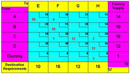
Table 7.3 shows a northwest-corner assignment. (Cell A-E was assigned first, A-F second, B-F third, and so forth.) Total cost : 10*10 + 30*4 + 15*10 + 30*1 + 20*12 + 20*2 + 45*12 + 0*1 = 1220($).
Inspection of Table 7.3 indicates some high-cost cells were assigned and some low-cost cells bypassed by using the northwest-comer method. Indeed, this is to be expected since this method ignores costs in favor of following an easily programmable allocation algorithm.
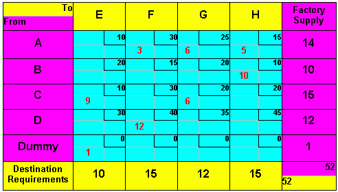
Table 7.4 shows a least-cost assignment. (Cell Dummy-E was assigned first, C-E second, B-H third, A-H fourth, and so on.) Total cost : 30*3 + 25*6 + 15*5 +10*10 + 10*9 + 20*6 + 40*12 + 0*1= 1105 ($).
Table 7.5 shows the VAM assignments. (Cell Dummy-G was assigned first, B-F second, C-E third, A-H fourth, and so on.) Note that this starting solution is very close to the optimal solution obtained after making all possible improvements (see next chapter) to the starting solution obtained using the northwest-comer method. (See Table 7.3.) Total cost: 15*14 + 15*10 + 10*10 + 20*4 + 20*1 + 40*5 + 35*7 + 0*1 = 1005 ($).

To develop an optimal solution in a transportation problem involves evaluating each unused cell to determine whether a shift into it is advantageous from a total-cost stand point. If it is, the shift is made, and the process is repeated. When all cells have been evaluated and appropriate shifts made, the problem is solved. One approach to making this evaluation is the Stepping stone method.
The term stepping stone appeared in early descriptions of the method, in which unused cells were referred to as "water" and used cells as "stones" from the analogy of walking on a path of stones half-submerged in water. The stepping stone method was applied to the VAM initial solution, as shown in Table 7.5
Table 7.6 shows the optimal solutions reached by the Stepping stone method. Such solution is very close to the solution found using VAM method.
7.4 Alternate Optimal SolutionsWhen the evaluation of any empty cell yields the same cost as the existing allocation, an alternate optimal solution exists (see Stepping Stone Method alternate solutions). Assume that all other cells are optimally assigned. In such cases, management has additional flexibility and can invoke nontransportation cost factors in deciding on a final shipping schedule.
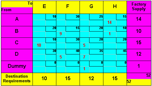
Table 7.7 "Alternate Optimal Matrix for the Chest Transportation Problem, With Minimum Transportation Cost of $1,000.
7.5 Degeneracy
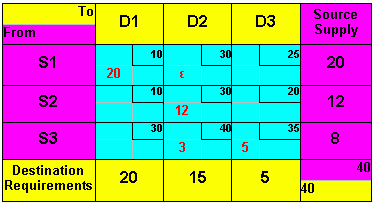
Degeneracy exists in a transportation problem when the number of filled cells is less than the number of rows plus the number of columns minus one (m + n - 1). Degeneracy may be observed either during the initial allocation when the first entry in a row or column satisfies both the row and column requirements or during the Stepping stone method application, when the added and subtracted values are equal. Degeneracy requires some adjustment in the matrix to evaluate the solution achieved. The form of this adjustment involves inserting some value in an empty cell so a closed path can be developed to evaluate other empty cells. This value may be thought of as an infinitely small amount, having no direct bearing on the cost of the solution.
Procedurally, the value (often denoted by the Greek
letter epsilon, - ![]() )
is used in exactly the same manner as a real number except that it may
initially be placed in any empty cell, even though row and column requirements
have been met by real numbers. A degenerate transportation problem showing
a Northwest Corner initial allocation is presented in Table 7.8, where
we can see that if
)
is used in exactly the same manner as a real number except that it may
initially be placed in any empty cell, even though row and column requirements
have been met by real numbers. A degenerate transportation problem showing
a Northwest Corner initial allocation is presented in Table 7.8, where
we can see that if ![]() were not assigned to the matrix, it would be impossible to evaluate several
cells.
were not assigned to the matrix, it would be impossible to evaluate several
cells.
Once a ![]() has been inserted into the solution, it remains there until it is removed
by subtraction or until a final solution is reached.
has been inserted into the solution, it remains there until it is removed
by subtraction or until a final solution is reached.
While the choice of where to put an ![]() is arbitrary, it saves time if it is placed where it may be used to evaluate
as many cells as possible without being shifted.
is arbitrary, it saves time if it is placed where it may be used to evaluate
as many cells as possible without being shifted.
7.6
Transportation Problem with a Maximization as a Criterion
A fictive corporation A has a contract to supply motors for all tractors produced by a fictive corporation B. Corporation B manufactures the tractors at four locations around Central Europe: Prague, Warsaw, Budapest and Vienna. Plans call for the following numbers of tractors to be produced at each location:
Prague 9 000
Warsaw 12 000
Budapest 9 000
Corporation A has three plants that can produce the motors. The plants and production capacities are
Hamburg 8 000
Munich 7 000
Leipzig 10 000
Dresden 5 000
Due to varying production and transportation costs, the profit earns on each motor depends on where they were produced and where they were shipped. The following transportation table (Table 7.9) gives the accounting department estimates of the euro profit per unit (motor).
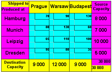
Table 7.10 shows a highest - profit assignment (Least Cost method modification). In contrast to the Least Cost method it allocates as much as possible to the highest-cost cell. (Cell Hamburg - Budapest was assigned first, Munich - Warsaw second, Leipzig - Warsaw third, Leipzig Budapest fourth, Dresden Prague fifth and Leipzig Prague sixth.) Total profit : 3 335 000 euro.
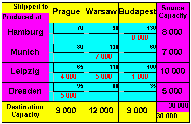
Applying the Stepping Stone method (modified for maximization purposes) to the initial solution we can see that no other transportation schedule can increase the profit and so the Highest Profit initial allocation is also an optimal solution of this transportation problem.
7.7 The Transshipment Problem
The transshipment problem is similar to the transportation problem except that in the transshipment problem it is possible to both ship into and out of the same node (point). For the transportation problem, you can ship only from supply points to demand points. For the transshipment problem, you can ship from one supply point to another or from one demand point to another. Actually, designating nodes as supply points or demand points becomes confusing when you can ship both into and out of a node. You can make the designations clearer if you classify nodes by their net stock position-excess (+), shortage (-), or 0.
One reason to consider transshipping is that units
can sometimes be shipped into one city at a very low cost and then transshipped
to other cities. In some situations, this can be less expensive than direct
shipment.
Let's consider the balanced transportation problem
as an example.
Picture 7.1 shows the net stock positions for the three warehouses and four customers. Say that it is possible to transship through Pilsen to both Innsbruck and Linz. The transportation cost from Pilsen to Innsbruck is 300 euro per unit, so it costs less to ship from Warsaw to Innsbruck by going through Pilsen. The direct cost is 950 euro, and the transshipping cost is 600 + 300 = 900 euro. Because the transportation cost is 300 euro from Pilsen to Innsbruck, the cost of transshipping from Prague through Pilsen to Innsbruck is 400 euro per unit. It is cheaper to transship from Prague through Pilsen than to ship directly from Prague to Innsbruck.
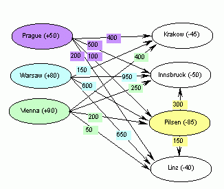
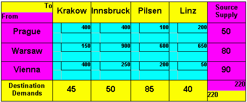
There are two possible conversions to a transportation model. In the first conversion, make each excess node a supply point and each shortage node a demand point. Then, find the cheapest method of shipping from surplus nodes to shortage nodes considering all transshipment possibilities. Let's perform the first conversion for the Picture 7.1 example. Because a transportation table Prague, Warsaw, and Vienna have excesses, they are the supply points. Because Krakow, Pilsen, Innsbruck, and Linz have shortages, they are the demand points. The cheapest cost from Warsaw to Innsbruck is 900 euro, transshipping through Pilsen. The cheapest cost from Prague to Innsbruck is 400 euro, transshipping through Pilsen too. The cheapest cost from all other supply points to demand points is obtained through direct shipment. Table 7.11 shows the balanced transportation table for this transshipment problem. For a simple transportation network, finding all of the cheapest routes from excess nodes to shortage nodes is easy. You can list all of the possible routes and select the cheapest. However, for a network with many nodes and arcs, listing all of the possible routes is difficult.
Another transportation problem is the assignment problem. You can use this problem to assign tasks to people or jobs to machines. You can also use it to award contracts to bidders. Let's describe the assignment problem as assigning n tasks to n people. Each person must do one and only one task, and each task must be done by only one person. You represent each person and each task by a node. Number the people 1 to n, and number the tasks 1 to n. The assignment problem can be described simply using a verbal model or using a linear programming mathematical model .
For example, say that five groups of computer users must be trained for five new types of software. Because the users have different computer skill levels, the total cost of trainings depends on the assignments.
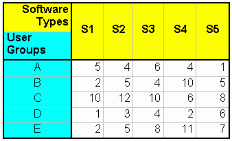
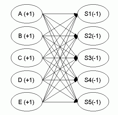
Table 7.12 shows the cost of training for each assignment of a user group (A through E) to a software type (S1 through S5). Picture 7.2 is a network model of this problem.
A balanced assignment problem has the same number
of people and tasks. For a balanced assignment problem, the relationships
are all equal. Each person must do a task. For an unbalanced assignment
problem with more people than tasks, some people don't have to do a task
and the first class of constraints is of the ![]() type. In general, the simplex method does not guarantee that the optimal
values of the decision variables are integers. Fortunately, for the assignment
model, all of the corner point solutions have integer values for all of
the variables. Therefore, when the simplex method determines the optimal
corner point, all of the variable values are integers and the constraints
require that the integers be either 1 or 0 (Boolean).
type. In general, the simplex method does not guarantee that the optimal
values of the decision variables are integers. Fortunately, for the assignment
model, all of the corner point solutions have integer values for all of
the variables. Therefore, when the simplex method determines the optimal
corner point, all of the variable values are integers and the constraints
require that the integers be either 1 or 0 (Boolean).
7.8.1 Conversion to a Balanced Transportation Table
It's not surprising that the variable values for corner point solutions to the assignment model are integers. The assignment model is a special case of the transportation problem, and the transportation problem has integer variable values for every corner point.
For the assignment model, the number of supply and demand points are both n. The supply points correspond to each person, and the demand points correspond to each task. Furthermore, every supply amount is 1 and every demand amount is 1. There is one of each person and one of each task.
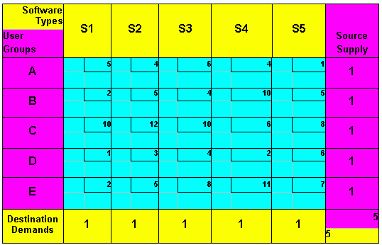
Table 7.13 The Computer Users Assignment Problem in the Transportation Table Format
Table 7.13 represents the computer users assignment problem in the balanced transportation table format. For the computer users assignment problem, you minimize the total cost of training. Because number of users = 5 and software types = 5, the transportation problem is balanced. You can use standard method for initial solution finding (Northwest-Corner method, Least-Cost method, or Vogel's approximation method (VAM) and a SteppingStone method for developing an optimal solution.
Thinking of the transportation problem as shipping items between cities is helpful, but it's the mathematical structure that is important. The assignment problem has the same mathematical structure as the transportation problem, even though it has nothing to do with shipping units.
Note, that each feasible solution of assignment problem will always be strongly degenerated (number of nonzero variables will always be n).
7.9 Conclusion
The transportation problem is only a special topic of the linear programming problems. It would be a rare instance when a linear programming problem would actually be solved by hand. There are too many computers around and too many LP software programs to justify spending time for manual solution.( There are also programs that assist in the construction of the LP or TP model itself. Probably the best known is GAMSGeneral Algebraic Modeling System (GAMS-General, San Francisco, CA). This provides a high-level language for easy representation of complex problems.)