Mathematical Model of the Shortest Route Problem

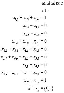
The decision variables are defined x_ij, The arc (i,j) is either included in the shortest route (x_ij = 1) or not (x_ij = 0).

We are searching for the shortest route from Prague to Singapore (Picture 8.6 in level 1).

For Node 1 (Prague) the net stock position is 1 and one of outgoing arcs (to Frankfurt, to Zurich or to Vienna) must be on the shortest route thus

For Node 9 (Singapore) the net stock position is -1 and one of incoming arcs (from Bangkok or from Dubai) must be on the shortest route too, thus

This equation can be multiplied by –1 and so

For nodes 2 to 8 the net stock position is 0 and the conditions are created in the same way as for Maximum Flow Problem.

Our objective is to minimize the sum of distances between the transition airports on the route, i.e. the objective function is
 
 

z = 410x_1,2 + 252x_1,3 + 526x_1,4 + 4830x_2,6 + 2442x_3,5 + 2878x_4,5 + 9026x_4,8 +

+ 2026x_5,6 + 6810x_5,8 + 1937x_6,7 + 5840x_6,9 + 3000x_7,8 + 1430x_8,9
 
 

The entire bivalent linear programming model is